Weak and strong coupling
For the discussion of the weak and strong coupling we consider again an S = 1/2, I = 1/2 system with an isotropic giso-value and isotropic coupling aiso > 0. We assume that the high field approximation is valid so that all spins, electrons and nuclei, are quantized along the direction of the magnetic field vector B0, taken along z. The magnetic field set up by the HFI at the nucleus is therefore directed along the z-axis. The energy levels of this system are obtained by setting B = 0 in Eq. (15).
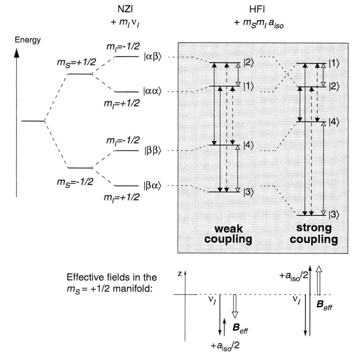
Fig. 6: (top) Energy level scheme for an S = 1/2, I = 1/2 system in the weak and strong coupling case together with the possible electron and nuclear spin transitions. (bottom) Schematic drawing of the effective magnetic fields set up at the nucleus by the superposition of the NZI and HFI for the mS = +1/2 manifold.
In Fig. 6, the energy level schemes are drawn for the weak and the strong coupling case. It is assumed that νI < 0 and aiso > 0. The electron and nuclear Zeeman levels are indexed by their magnetic quantum numbers mS and mI and commonly designated by |αα>, |αβ>, |βα> and |ββ>, where |α> and |β> refer to the two spin state in the external magnetic field. In general mI is not a good quantum number for the characterization of the energy levels since the quantization axis of the nuclear spin deviates from the direction of the external magnetic field due to the HFI. For this reason a new numbering of the levels is introduced, namely |1>, |2>, |3> and |4>. The numbering of the levels in the weak and strong coupling case is shown in the figure.
In the weak coupling case (νI > aiso/2) the direction of quantization of the nuclear spin is given in first order by the external magnetic field B0. This is illustrated in the vector diagram at the bottom of Fig. 6 for the mS = +1/2 manifold. The magnetic fields put up by the NZI and the HFI are drawn along the z-axis and have opposite directions. The effective quantization vector, experienced by the nucleus and indicated by the bold arrow, is obtained by the addition of both contributions. The hyperfine field slightly decreases the energy splitting caused by the NZI.
In the strong coupling case (νI < aiso/2) the direction of quantization of the nuclear spin is determined by the hyperfine field aiso/2. The NZI gives only a small contribution to the effective field. Again the fields act in opposite directions in the mS = +1/2 manifold.
In the mS = -1/2 manifold, the nuclear Zeeman and hyperfine fields act in the same direction for both weak and strong coupling. The splitting between the Zeeman states is thus increased as can be inferred from the energy level diagram in Fig. 6.
We now consider the more general case where additional terms in the spin Hamiltonian cause the quantization axis to deviate from the z-axis. This is e.g. the case when the high-field approximation is no more valid and Sx and Sy have to be considered or when the coupling is anisotropic (B <> 0). As a result not only the magnitude of the effective field experienced by the nucleus but also the direction is changed when going from one mS to another. This has important effects on the transition frequencies observable in the four level system as a change in the mS spin state can now also affect the spin state of the nucleus. The transition probability of the so-called forbidden transitions increases. In Fig. 6 the six possible transitions between the four levels are indicated both for the weak and strong coupling case. The allowed electron transitions, involving only a spin flip of the electron (ΔmS = ±1, ΔmI = 0) are indicated by full arrows, the forbidden electron transitions where both the electron and the nuclear spins flip (ΔmS = ±1, ΔmI = ±1) by dashed arrows. The hollow arrows represent the nuclear transitions which take place within the mS manifolds. Note that in our example with isotropic coupling the forbidden transitions have zero transition probability.
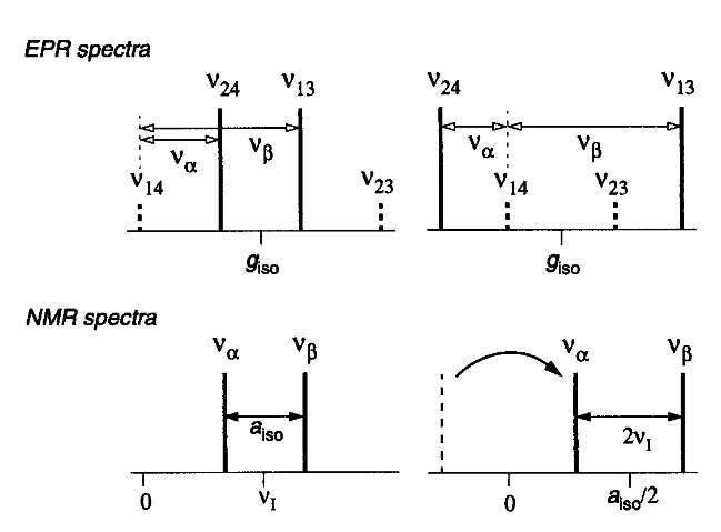
Fig. 7: (top) EPR stick spectra observed for the energy level schemes in Figure 6 for the weak and strong coupling case. The allowed and forbidden electron transitions are drawn as solid and dashed lines, respectively. The nuclear frequencies are indicated as energy differences between the electron transitions. (bottom) Corresponding NMR spectra with positive frequencies only.
The EPR and NMR spectra, obtained for the energy level schemes in Fig. 6, are drawn schematically in Fig. 7 for the weak and strong coupling case. In the EPR spectrum allowed (solid lines) and forbidden (dashed lines) transitions are centered around giso. The numbering of the frequencies is taken from the energy level scheme with νij = Ei-Ej. The nuclear transition frequencies να and νβ are shown as energy differences between the allowed and forbidden transitions. They are given by the absolute values of the transition frequencies ν12 and ν34. In the NMR spectrum in Fig. 7 only positive frequencies are observed with the consequence that να and νβ are centered around aiso/2 and separated by 2νI in the strong coupling case.
The intensities of the allowed and forbidden electron transitions are given by
$$ I_{a} = \text{cos}^2\eta = \frac {\left|\nu^2_I - \frac {1}{4}\nu_{-}^2\right|} {\nu_{\alpha}\nu_{\beta}} \ \qquad (21 a)$$
and
$$ I_{f} = \text{sin}^2\eta = \frac {\left|\nu^2_I - \frac {1}{4}\nu_{+}^2\right|} {\nu_{\alpha}\nu_{\beta}} \ \qquad (21 b)$$
where ν+ = ν12 + ν34 and ν- = ν12 - ν34. The angle η is the half sum of the angles between the external magnetic field and the effective field vectors acting on the nucleus in the two mS manifolds. It is obtained by the diagonalization procedure of the Hamiltonian in Eq. (15) and has to be chosen as -45o < η ≤ 45o for the numbering of the levels in Fig. 6 to be correct. From these formulae it can be seen that for η = 0 (all fields along z as in Fig. 6) the intensity of the forbidden transitions is zero.